Context
Radio astronomy is the study of celestial objects at radio frequencies: in the electromagnetic spectrum, from 20 kHz to 300 GHz. It differs with optical astronomy where we look in the visible part of the EM spectrum or close infrared/ultraviolet range (i.e. electromagnetic waves it the hundreds of THz).
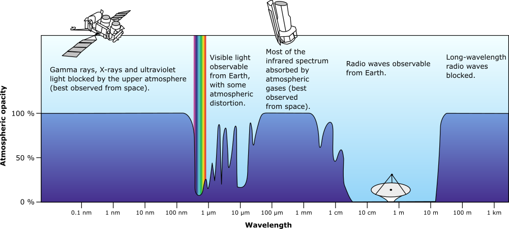 Plot of Earth's atmospheric opacity to various wavelengths of electromagnetic radiation, by NASA, Public Domain, on wikimedia
At these lower frequencies, the wavelength (λ) is much longer: 2.7 cm in my case (Ku band), compared to hundreds of nanometers with optics. This inherently limits our resolving power even with massive antennas. To improve resolution, interferometry is used: an array of sensors, which can be continents apart are coupled.
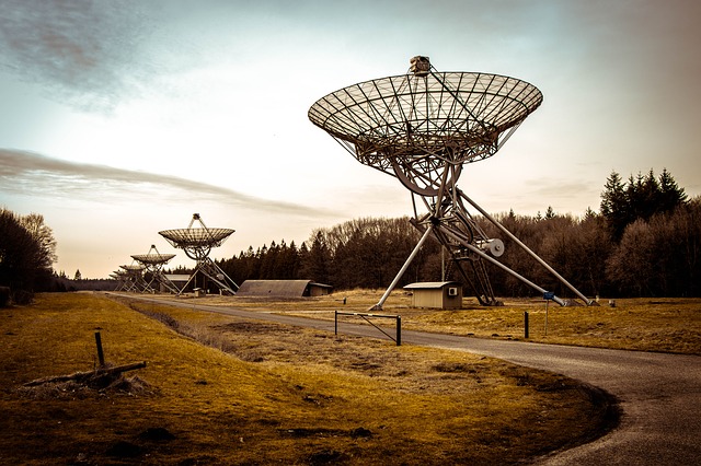 Westerbork Synthesis Radio Telescope, an aperture synthesis interferometer in the northeastern Netherlands.
The point of looking at various astronomical phenomenon in this frequency range is that they have different origins and/or propagation properties. Also, due to the cosmological red-shift (caused by the expansion of the universe), some radiation emitted at a much higher frequency ends up in this range. This is the case of the Cosmic Microwave Background, for instance.
Radio waves are less affected by interstellar dust, the Earth's atmosphere and meteorological conditions (depending on the frequency). The physical construction of antennas is also less demanding that optical instruments: the accuracy must be a fraction of the wavelength i.e. a few centimeters for VHF compared to nanometers in optics. This means that we can build massive radio telescopes such as the Five-hundred-meter Aperture Spherical radio Telescope (FAST) in China. This scale would not be feasible for an optical mirror.
This graph shows the main natural radio sources in the sky and their flux density versus the frequency. The vertical line is the center frequency of my setup.
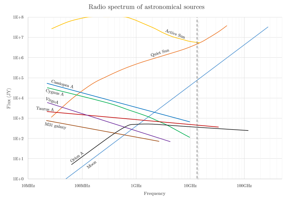 Radio spectrum of astronomical sources, CC BY 3.0, based on data from portia.astrophysik.uni-kiel.de
An amateur astronomer with a very simple and inexpensive setup can perform some interesting measurements. This is mine:
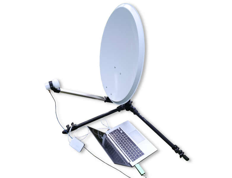
This allows me to survey the sky in Ku radio band: from 10.7 to 12.75 GHz. Although this band is quite busy due it being used for satellite communications (notably satellite TV), there are two big advantages: the hardware is very easy and cheap to get, and the parabola can be small for a given resolving power/gain due to the short wavelength.
In this article, I describe this setup and some experiments we can do with it.
The acquisition chain
This is a block diagram of my acquisition chain:
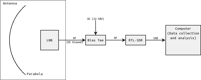
In the following section, I will describe every element of this acquisition chain and how they interface.
Parabolic reflector
The most noticeable element of our antenna is the parabolic reflector, commonly referred as a dish. It reflects incoming electromagnetic radiation into the feed horn of the LNB (see below).
A parabola (or paraboloid for the revolved 3D shape) has the unique property of having a focus point, where light entering it traveling parallel to the axis of symmetry is reflected toward the focus with an identical travel length.
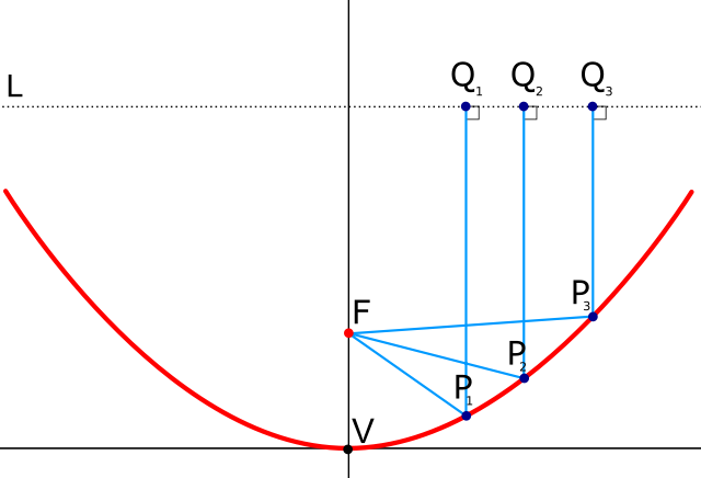 Parabolic reflector properties, Public Domain, on wikimedia
If a sensor is placed at the focal point of the parabola so that its radiation pattern covers the area of the dish, it effectively acts as a very high gain and highly directional antenna.
This picture shows the typical radiation pattern of a parabolic antenna, where hotter colors means more gain.
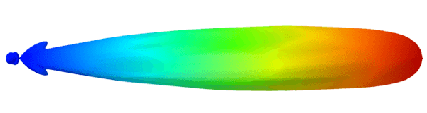 3D radiation pattern of a parabolic antenna, determined using a simulation program, by Christian Wolff, CC BY-SA 3.0, on radartutorial
At any given frequency, a larger dish will give us more directivity (i.e. more signal power) and a better angular resolution, which are both highly desirable for RA. Therefore, we want the largest dish possible. The limitations are of course cost, and ease of use to aim at astronomical objects (mass and size).
Indeed, the formula to get the approximate angular resolution in radians is:

And the maximum gain of the main lobe is:
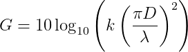
k is the efficiency factor which is generally around 60% for an off-set parabola.
For my system, I chose an elliptical dish made by Engel, dimensions 550×600 mm (angular resolution of 2.6° by 2.8°). It is designed for Ku band satellite TV reception, and has an off-set construction: the feed horn is not is the way of the wave, which improves efficiency. I bought it at a local hardware store for 30€ with the LNB and mounting hardware included.
Low Noise Block (LNB) and power supply
The central element of our acquisition chain is the Low-Noise Block (LNB). Not only does it contains the actual antenna that collects the energy of the wave focused by the parabola, but it also shifts it to a lower frequency and amplifies it so that we can measure it. It uses the superheterodyne principle to achieve this, by mixing the input signal with a local oscillator (LO). The advantage of performing this transformation directly after the antenna is that the lower frequencies travel through coax cable with much lower attenuation.
My LNB is an Engel AN7123. This is my LNB fitted with an F to SMA adapter:
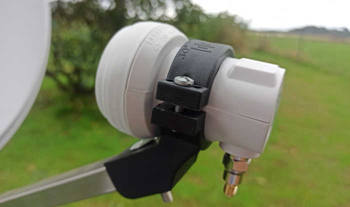 Engel AN7123 LNB on my parabola
LNBs have several important characteristics to consider:
- Input and output frequency range: they are standard, described below.
- Amplifier gain: usually 50 to 65 dB (55 dB for mine).
- Noise figure: the signal to noise ratio at the input divided by the signal to noise ratio at the output. Usually between 0.1 and 0.2 dB. It can be converted to a noise temperature with this formula:

This temperature is our noise floor when no radio source is in the main lobe. 0.1 dB corresponds to 7 K. This will be important for our measurements.
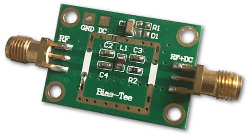
A LNB has some active circuitry to perform those operations. It needs a power supply. It is powered through its RF output, by adding a DC bias. Hence, we need to add a biasing circuit between the LNB and the receiver, like this one:
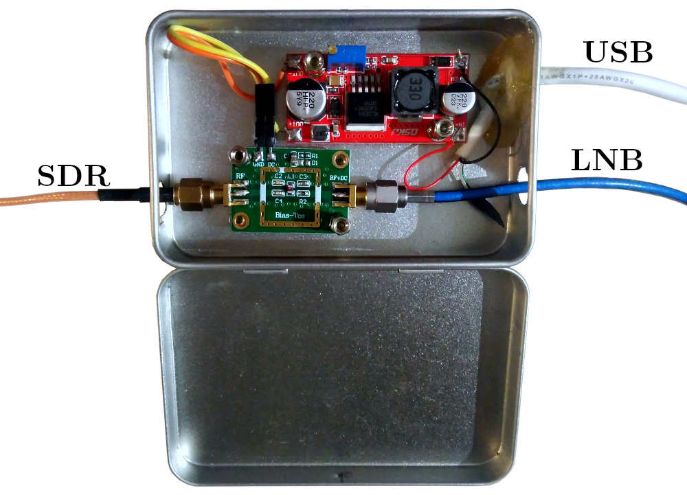
To power the bias-tee, I use 5 V USB from my computer with a XL6009 DC-DC boost converter module in order to get the voltage in the adequate range. A potentiometer can be trimmed to adjust the output voltage.
I enclosed this circuitry in a shielded metal box:
The LNB uses a vertically polarized antenna if the DC supply voltage is between 11 V and 14.5 V, and horizontally polarized if it is between 15.5 V and 22 V. Additionally, the input/output frequency range is selected by the presence/absence of a 22 kHz tone:
- With no tone, the local oscillator (LO) is f=9.75 GHz, input range 10.7 to 11.7 GHz and output range 950 to 1950 MHz.
- With a tone, the local oscillator is f=10.6 GHz, input range 11.7 to 12.75 GHz and output range 1100 to 2150 MHz.
The formula to get the actual frequency from a measurement is simply:

The temperature stability for these LNBs is pretty bad, meaning that for narrow band work, a warm-up time is required. This is also the case for the receiver.
The LNB may be replaced with a C band (3.5 to 4.2 GHz) one, which can also be found for cheap online because it is used for satellite TV in certain parts of the world. This is interesting because objects behave differently at different frequencies as shown in the graph above. However, the drawback is that we need a parabola about twice as big to get the same directivity. My parabolic reflector is too small to achieve anything in the C band. A meter in diameter is a minimum for this band.
Measurement hardware (SDR)
The "old way" to measure the signal output was to use a satellite finder, and modify it to fit an analog-to-digital converter. This only gives a power measurement (magnitude) over a broadband. It is 1D data.
The "new way" is to use a Software Defined Radio or SDR. In my case, I used a RTL-SDR receiver with a TCXO (temperature compensated crystal oscillator). This outputs much richer data (I/Q samples) over a bandwidth of up to 3.2 MHz, from 24 MHz to 1766 MHz. With this raw data, we can compute the power spectral density, demodulate signals, etc. The only "drawback" is that to use the complex data, we need to use and/or write signal processing software (with GNU Radio, for instance).
Note on impedance matching: the LNB and RTL-SDR are 75 Ω terminated. However, we are using 50 Ω coax and tee-bias. This mismatch will cause some losses which results in reduced signal to noise ratio. However, the mismatch loss when using 50 Ω cabling on a 75 Ω input will be less than 0.177 dB. Realistically, this will have a minimal influence on the measurements (the signal is already amplified by the LNB well above the SDR's own noise floor).
The software
As described above, using RTL-SDR, we can get a lot of data (up to 3.2 mega samples per second). The last step is to process this data with signal processing software. With a single antenna, we are mostly interested with the power spectral density (magnitude vs. frequency).
The RTL-SDR's drivers provide a tool to do this: rtl_power. It outputs CSV files. I process this data with Python scripts (using scipy, numpy and matplotlib).
All of my code is available on my Github/rtl_power_scripts.
I also use the following open-source software to prepare the measurements:
- rtlSpectrum (Apache License 2.0),
- Gqrx (GNU GPL v3),
- rtl_power_fftw (GNU GPL v3).
Experiments
In this section, I will be detailing some measurements that can be performed with this radio-astronomy setup.
Power spectral density
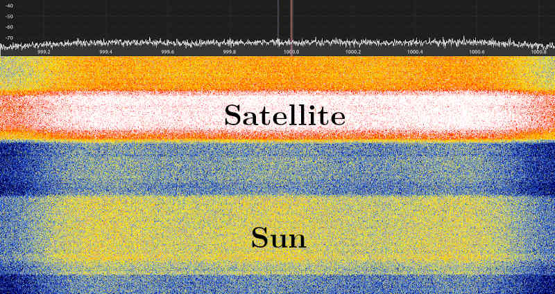
With the RTL-SDR reciever, we can perform a broadband scan and get a PSD (power spectral density) plot.
To aim the parabola at objects, I use GQRX. This screenshot shows the waterfall plot: the horizontal axis is frequency, the vertical axis is time and hotter colors means more signal power. Here, the parabola was aimed at the sun, and then at a TV satellite.
The position of objects that are not visible to the naked eye (such as geostationary satellites) can be obtained using the open-source software Stellarium. Using a smartphone's gyroscope as a 3D inclinometer is enough to get a fairly accurate estimation of the current azimuth and elevation of the parabola. This requires calibration with a known source, such as the sun, to get an offset angle on both axes.
Once the object is centered, we can use rtl_power to get the data:
rtl_power -f 950M:1500M:128k -i 120 -g 0 output.csvI used Python to plot this data:
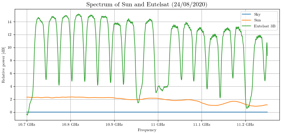
The sky measurement is used a a baseline to remove the average noise for each frequency bin (hence the "relative" nature of the plot).
The Sun spectrum is mostly flat which is to be expected because of its thermal nature. The slight dip at higher frequency is probably due to error in measurements.
Note: to compensate for bad data on the edge of the bandwidth of each frequency hop, I used a two stage Savitzky-Golay filter implemented in a Python. A better way to avoid this effect is to use the "crop" parameter of rtl_power, that ignores this data altogether. The drawback is that is increases the number of frequency hops for a given bandwidth.
Capturing a Sun transit
For this experiment, the parabola is aimed so that the sun is perfectly in the center of the field at t=0. The position of the parabola is then locked in place so that the Earth's rotation slowly cause it to go out of the main lobe. This way, we capture half of a Sun transit through the field of the parabola. To capture the data, I used my power measurement tool with this command:
python3 -u SDR_measure.py -i 100 -f 1000 -g 10 > output.csvThis is the filtered result plotted with Matplotlib:
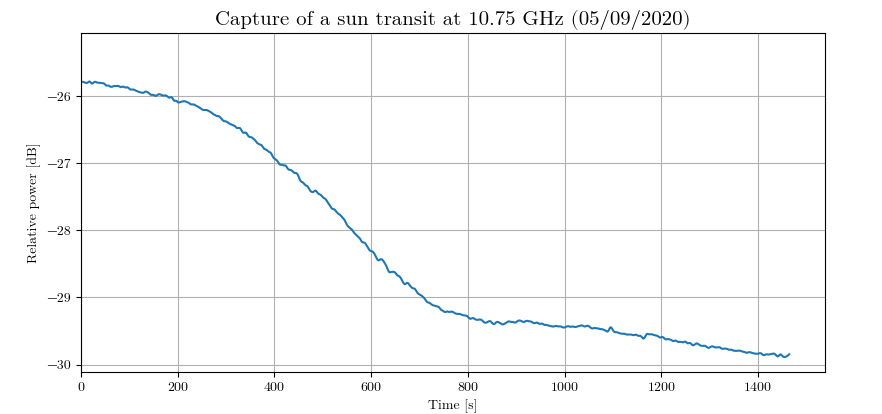
The equation to get the half power point is:

According to our graph, the Sun's level reaches this half power mark in about 7 minutes after being placed in the center. Given that the half-power beamwidth (HPBW) should be about 2.8° according to the previous calculations, we can compute the expected time to reach this level, because we also know the rotation speed of the Earth:
![T_{transit} \text{ [min]} = \frac{\Theta \times 24 \times 60}{360}](/projects/20200907_Radio_astronomy_basics/equation_transit_time.png)
According to this equation, this expected time is about 10 minutes, i.e. 5 minutes for half the transit. Our measurement is a bit higher than the expectation. This means that the main lobe is wider than the estimation.
Interestingly, we see a smaller bump in the graph after the main one: at t = 1000 s. It is probably caused by the Sun being captured by the side lobes of the antenna.
Measuring the Sun's temperature
Following the previous measurement, the parabola was also aimed at the ground, and at Eutelsat 3B:
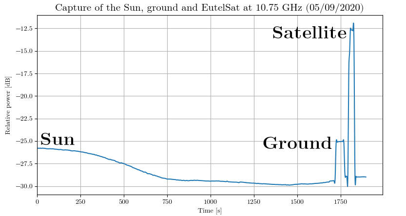
Using this data, we can estimate the temperature of the Sun.
Apart from artificial satellites broadcasting in the Ku band, most of the energy we capture is black body radiation. By measuring two additional points (the ground and a point at the zenith), knowing their temperature, we can establish a calibration curve. This is my data for the previous graph:
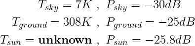
The equation for the calibration curve can then be computed with a linear regression between those points:

P is the linear power (not in decibels) and T the temperature in Kelvin. If we plug in our numbers, we get T = 226.5 K for the Sun.
We then need to account for the fact that the sun only occupies a fraction of the field of view of the parabola.
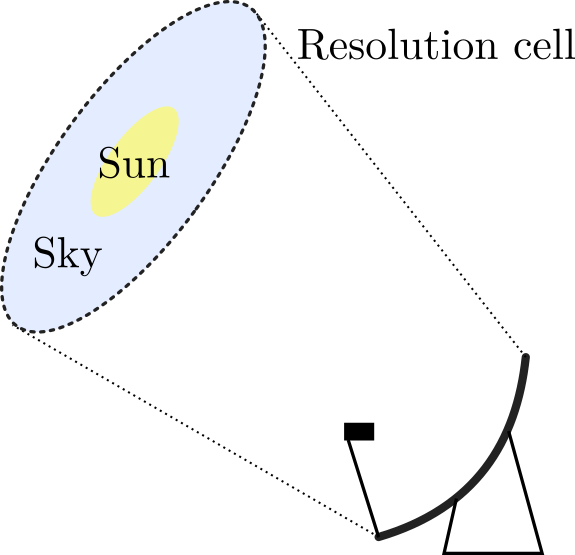 Size of the Sun relative to the resolution cell of the antenna
This effectively means that our measurement is an average of every source of radiation in the resolution cell. Therefore, we need to compute a dilution factor, which is the ratio between the solid angle subtended by the lobe of the parabola and the solid angle the Sun subtends. This depends on the dimensions of the parabolic reflector and the frequency. The calculations are:
With my parabola (55×60 cm), I get a dilution factor of about 25.5 for the Sun: it fits twenty five times and a half within the main lobe of the parabola. We can estimate its actual temperature by compensating for that effect. If we suppose that the gain is uniform and that the only other source of radiation in the lobe is the background cold sky, the equation is:

Hence, we get T = 5984 K. This temperature is about right: we expected about 6000 K.
There are several sources of error in this calculation; some of which may compensate each other:
- The lobe is probably larger than this calculated value, as we saw in the transit plot. We probably underestimated the dilution factor.
- There is some atmospheric absorption. Ku band is right at the limit of the atmosphere's transparency frequency limit.
- The parabola and LNB get hot themselves, especially when directly facing the sun. Filtering got rid of a huge spike in power at t=0s.
- We suppose that the gain is uniformly distributed in the main lobe, whereas it is actually higher in the center, and gradually lowers to -3dB. This effect could be compensated if we knew the radiation pattern of the parabola.
- The radiation pattern has side lobes, which bias the measurements.
Radio source mapping
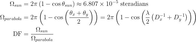
The parabola is on a azimuth-elevation mount. If we change these angles while recording their value and the current power density, we can a 2D power map of the sky. This idea is somewhat similar to my previous project "Electromagnetic interference mapping".
To record the angles, I attached an Android phone to the parabola's arm with the app Physics Toolbox Suite. It includes, among others, an inclinometer with CSV logging.
This graph shows the time-correlated power, azimuth and elevation angles.
The data is post-processed with a Python script to do the time correlation, noise filtering, drift compensation and plotting with Matplotlib. Those parameters are currently manually determined.
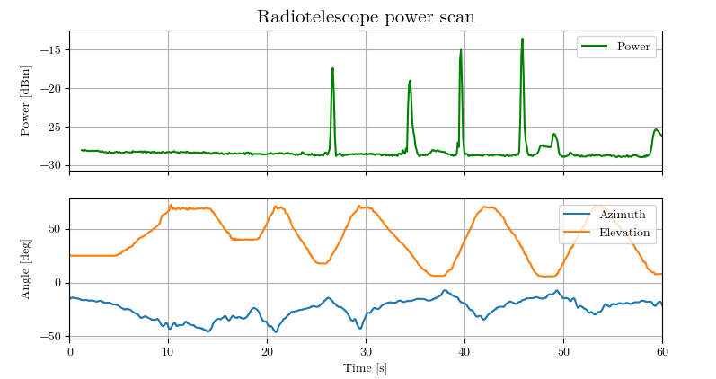
This is a power map, centered on the sun (at 33° elevation):
The lighter spots at elevation 10° are trees.
This technique is a work-in-progress, and has two major issues with the inclinometer readings:
- Noise: there is a ±1° noise of both axes measurements. Savitzky-Golay filtering works great here.
- Drift: the angle is obtained by integration of the gyroscope. This introduces a drift if the values are biased. The pitch/elevation angle can be compensated by using a complementary filter with the accelerometer. However, the yaw/azimuth angle is trickier to handle. Unfortunately, this drift depends on temperature, pressure, etc.
An obvious solution is to use a motorized mount instead, but this is much more expensive to make, and defeats the purpose of this experiment. I have several ideas to try to improve this technique in the future.
Conclusion
Using this setup, there is already a lot of experiments and measurements we can perform. There are also some improvements that we could do to get more interesting results:
- Use 2 parabolas or more to do interferometry,
- Mounting the parabola(s) on a motorized equatorial mount to follow the solar activity for instance,
- Use a different antenna in another electromagnetic band to look at different phenomenons (for instance, a VHF Yagi to listen for meteors).
Sources and links
- J.Köppen (2013, April). Fundamentals of Radio Astronomy, from https://portia.astrophysik.uni-kiel.de/~koeppen/10GHz/basics.html
- Jean Marie Polard F5VLB (2016). Amateur Radio Astronomy, from http://www.astrosurf.com/luxorion/Documents/amateur-radioastronomy-f5vlb-jm-polard.pdf (ebook)
- Peter Joseph Bevelacqua (2009). The Parabolic Reflector Antenna, from http://www.antenna-theory.com/antennas/reflectors/dish.php
Author: Charles Grassin
What is on your mind?
Sorry, comments are temporarily disabled.
#1 RF
on August 20 2023, 4:47