AI-powered digital signal processing

Context

Machine learning (ML) is a category of algorithm that allows software applications to become more accurate in predicting outcomes without being explicitly programmed. It relies on statistical analysis to build up a model.

Artificial neural networks (ANN) are the most commonly used models for machine learning. They are a group of interconnected nodes, with each connection having a weight. The learning process "simply" consist of optimizing those weights using mathematical operations such as gradient descent. Once those parameters are fixed (which may require very large data sets, depending on the complexity of the task), an output can be predicted for any input.

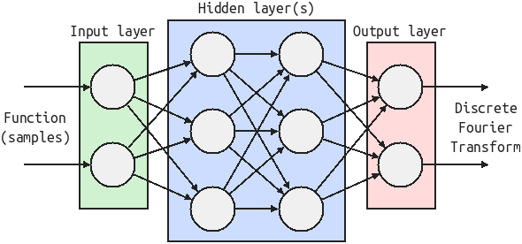An artificial neural network model, consisting of an input layer, some hidden layers and an output layer

Having an interest in digital signal processing (DSP), I wanted to share two machine learning experiments to perform tasks:

• Fourier transforms computation,
• Analog signal corruption recovery.

1. AI-powered Fourier transforms?

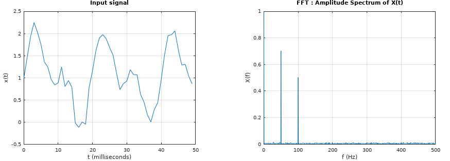
The discrete Fourier transform (DFT) converts a finite sequence of equally-spaced samples of a function into a function of frequency. There are widely used for applications in engineering, science, and mathematics. The fast Fourier transform (FFT) is an algorithm that computes the DFT of a function. Although FFTs are much faster than the naive implementation of DFT formula, they still take computing time, especially with very large data sets.

Raphaël Casimir submitted the idea that an ANN trained to do DFTs might be able to do it more efficiently than the FFT algorithm. Some error is acceptable since we are usually more interested in the peaks that the general noise content.

Hence, the question is: Can we use an artificial neural network trained with machine learning to compute Fourier transforms faster than the FFT algorithm?

Implementation

The basic building/training process for supervised ML is:

0. Build a neuron network model (i.e. programmatically specify the layers, activation functions, neurons types, loss function, etc.),
1. Train the model on a data set with known result (in this case, randomly generated periodic functions and their DFTs, computed by the standard FFT algorithm),
2. Use the trained model on some other data set with known result to check its predictions,
3. If the predictions are not satisfactory, repeat, adjust the model.

The amount of available data in the training set is often a limitation for machine learning. The fact that we can generate as much arbitrary data as we want in this case makes the whole process much easier!

My code is available on Github: ml_fourier_transform.py at CGrassin/DSP_machine_learning. I used Python 3 with TensorFlow. TensorFlow is an open-source software library for machine learning applications such as neural networks, originally developed by researchers and engineers working on the Google Brain team.

Result

I trained the model on 10,000 periodic functions, generated using the Fourier series formula and completely random coefficients. Then, we can test some predictions with functions generated using different parameters:

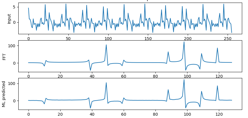
The top graph is the 128 samples input, the middle one is its standard FFT output, and the bottom one is the prediction of my model... this looks identical! I measured the RMS error for a test set of random functions, and consistently got less than 0.5% error.

The next thing I checked is the computation time, versus the Python implementation of FFT (numpy.fft.rfft). When looking at the time efficiency of a algorithm, it makes more sense to look at the time complexity rather that the mean execution time for a given input dimension. The time complexity shows how the execution time grows with more input data.

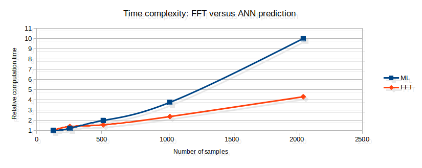
The FFT complexity is O(N×log(N)), meaning that an FFT computation for a dataset of size N points will have a worst time excecution time of t<λ×N×log(N). Unfortunately, my ML complexity seems quadratic, which is definitely not better that the FFT. This makes sense, because there are N×N/2 connections in my model; the complexity is therfore O(N²).

Having a look at how the model actually computes the DFT (the weights), this makes perfect sense: what it actually learned is the classic DFT formula!

Still, it is a nice representation of how a learning process can be implemented. It is impressive that Tensorflow was able to learn how to compute DFTs with close to zero error, while only training for only about 20 seconds on a very low power CPU (Core 2 Duo P7550 @ 2.26GHz)!

2. Data corruption recovery?

This second experiment is much more interesting: the idea is to attempt data recovery on an altered analog signal. I will be corrupting a waveform, and training an ANN to retrieve the original data. This is an example of what I want to feed in the ANN:

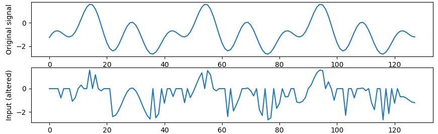
This would be very hard to recovery with a classical algorithm: we have to find the frequency, stitch the periods together and find a way to figure out all the points that are completely absent... Hence, ML is the perfect candidate for this task.

The implementation is similar to the one previously described, with a more complex ANN structure: 5 layers of N neurons, with a mix of linear and non-linear activation functions. Hence, the learning time is longer, and there is a higher risk of overfitting. To counteract this, I take a large input data set.

The python code is available in the same Github repository: ml_corruption_recovery.py.

Result

The model gets trained on 10,000 corrupted random periodic functions. It takes more time to converge, due to the number/complexity of the layers. This is the result:

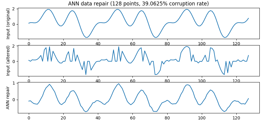
This result is impressive! The top plot is the original function, the middle one is the corrupted version (input for the ANN) and the bottom one is the repair attempt performed by the ANN. The waveform of the repair looks nearly identical to the original function, despite the high degree of alteration.

An interesting observation is that, even though the model was only trained with corrupted functions, feeding a non-altered function result in very small deformations, as shown is the following figure.

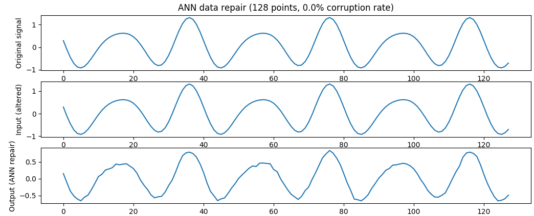
I am sure that this ANN could have some application in places where the alterations that a signal undergoes seem unpredictable, and very difficult to filter out with classic algorithms. However, there are some limitations: the network is not able to repair functions with discontinuities. A more complex model, perhaps using more advanced neuron types may be able to deal with this issue.

Takeaway

TensorFlow with Python are great for quick machine learning prototyping. Some prior theoretical ML knowledge is required to get started, but once this is figured out, it is very fast to put an ANN together, train it, a tweak the model.

I was able to quickly put together those two experiments. The results of the waveform recovery in particular are impressive as this would be extremely difficult to implement with traditional algorithms, as opposed to the 2 minutes it took to train the ANN to perform this task. I am only starting on ML, but I will definitely be trying much more in the future.