Context
Since the beginning of the space race in 1957, the number of objects sent into orbit is continuously growing, as does the amount of space debris orbiting the Earth. This is becoming a real threat for operational space missions around the Earth. Space debris can be the result of:
- A collision between two satellites, two debris or a satellite and a debris/meteoroid
- A battery which became unstable and exploded
- Fuel leftovers in a satellite or a launcher stage which became unstable and exploded
- A planned destruction
- An out of control satellite or a launcher stage
Today, the population of space debris is estimated to be more than 500 000 trackable objects where 20 000 of them are bigger than a tennis ball. In addition, there are millions of pieces too small to be detected.
The vast majority of space debris is located in Low Earth Orbit (LEO) where most space missions are located or planned.
 Representation of the distribution of the space debris in LEO in 2013. Source: ESA.
The ECE3SAT project is a student project developed at the french engineer school, ECE Paris. The goal of the project is to send a CubeSat in space to verify a physical theory permitting a fast deorbiting.
A CubeSat (1U-class spacecraft) is a nanosatelite satellite for space research that is made up of multiples of 10x10x11.35 cubic units, with a weight less than 1.33 kilograms. CubeSat are most commonly put in low Earth orbit by deployers on the International Space Station (ISS).
The Attitude Determination and Control System (ADCS) is focused on the control of the rotating motion of the satellite. Through sensors it will determine the attitude and act using it’s environment to reach the required orientation.
To test and validate the ADCS of the CubeSat, the team decided to build a device that can generate a steady and controlled magnetic field: a Helmholtz coils magnetic simulation environment.
Video
This video outlines the design, build and tests of our Helmholtz coils magnetic environment:
Objectives
Satellites may use the geomagnetic field (the Earth's magnetic field) for two purposes:
- Attitude determination with magnetometers,
- Attitude control with magnetorquers.
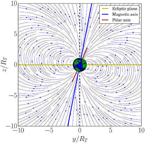 Geomagnetic field lines in the dipole approximation [1]
A magnetorquer is a device that creates a magnetic field which interacts with an ambient magnetic field in order to produce torque. For a coil of wire, the equation is:

Where τ is the resulting torque, μ is the permeability of the core, I is the current intensity, S is the oriented surface and B the ambient magnetic field. Note that due to the presence of a vector product, the torque can only be orthogonal to the geomagnetic field.
The major advantages of magnetorquers is that they are solid state (i.e. without moving mechanical parts) and only require electrical energy to run, which can be provided by onboard solar panels. However, they have a very low torque due to the low magnitude of the geomagnetic field. They are often used on small satellites due to the low torque they are able to generate in comparison to reaction wheels or cold gaz thrusters for instance.
Alternatively, some CubeSats use permanent magnets instead of coils (2D stabilization).
Having a system that allows us to generate arbitrary 3D magnetic fields gives the ability to perform physical tests of the nanosatellite.
What are Helmholtz coils?
Helmholtz coils are a pair of coils facing each other as shown in the scheme below.
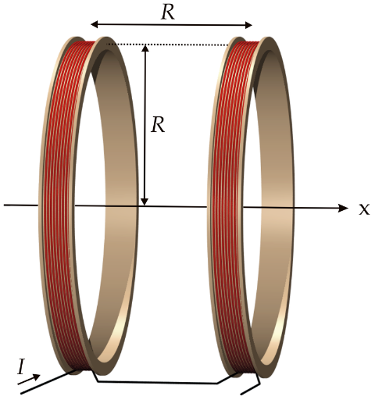 Helmholtz coils by Ansgar Hellwig, CC BY-SA 3.0, https://commons.wikimedia.org/w/index.php?curid=193184
This combination can generate a magnetic field between the two coils that is almost uniform on one axis. This is a spatial representation of this magnetic field on a plane orthogonal to the coils.
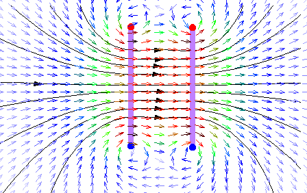 Helmholtz coils field by DVoigt, CC BY-SA 3.0, https://commons.wikimedia.org/w/index.php?curid=809676
The norm of this field depends of the radius of the coils, the number of windings and, more importantly, the intensity of the electric current. This means that, by controlling the amperage, we can chose the magnitude of the magnetic field according to this formula:

In order to achieve a three dimensional magnetic field, we use three pairs of Helmholtz coils, orthogonal to each other.
By building a device like this, it is possible to generate a magnetic field with a control on the norm and direction using the current. Thus we can:
- Test and calibrate magnetometers in a controlled environment,
- Test and validate the sizing of the magnetorquers,
- Integrate those two subsystems in a CubeSat model to test our filtering and positioning algorithms (Kalman, B-dot, etc.),
- Build a visual representation of the CubeSat's progress.
Design & Construction
The following section describes the design and construction of our Helmholtz simulation system.
Sizing
These were our design specifications:
| Requirement | Value |
|---|---|
| Volume of the constant filed zone | 64L (40x40x40cm) |
| Output magnetic field range | -5 to 5 Gauss |
| Input voltage range (per coil) | 20V to 60V |
| Max. input current (per coil) | 3A |
| Coils equivalent series resistance (ESR) | 22.5Ω |
| Time of assembly and disassembly | Less than 5 min. |
| Maximum variation of the field | < 10µT |
To meet those, we used the Wolfram Square Helmholtz Coils demonstration by Peter Euripides.
This is a simulation with 80 windings, with 80 cm square Helmholtz coils at 1.5 A:
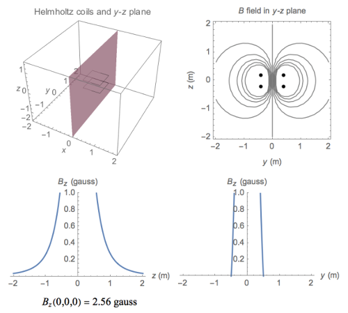 Wolfram simulation of the square Helmholtz coils with 1.5A
With this configuration, we get an amplitude of 5 Gauss (five times the geomagnetic field in each direction). By putting a current of 3A per coil instead, this rises to 10 Gauss, but it requires twice the input voltage.
Mechanical build
As discussed earlier, we chose the following dimensions for our simulator: 80 cm square coils with 80 turns. This adds up to about 256 m of copper per coil. The wire used for the winding is 0.5 mm (AWG 24) diameter copper enameled magnet wire.
To wind these coils, the frame is made out of aluminum profile, U-shaped. The outside width of the profile is 7.5 mm, which is enough to fit about 140 turns of our wire. It is also fairly rigid and inexpensive.
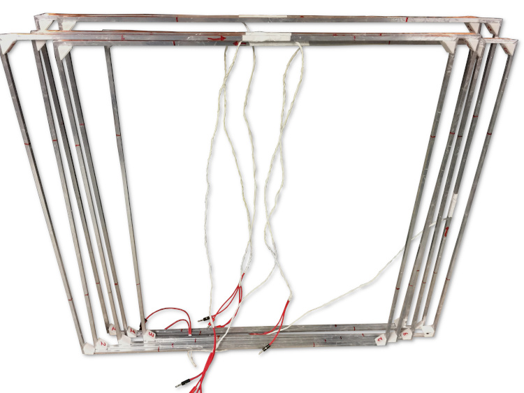 The 6 square coil frames when the cage is disassembled
The pairs of coils fit into each other. Numbers and arrows respectively indicate the size of the coil (80 mm, 78.5 mm and 77 mm) and the direction of the copper winding for quick assembly.
A jig was used to coil the wire, but this is by far the most time-consuming process of the build. Packing tape was added on top to protect the turns. The ends were terminated with 4 mm jacks.
In order to ensure that the assembly and disassembly time meet our constraints, we designed a 3D-printed clip that attaches the 6 coils of our Helmholtz simulator.
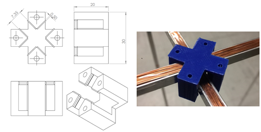 The 3D-printed clip design
This part could be swapped for a more definitive mounting method if need be.
This is the assembled Helmholtz magnetic simulation system with the clips:
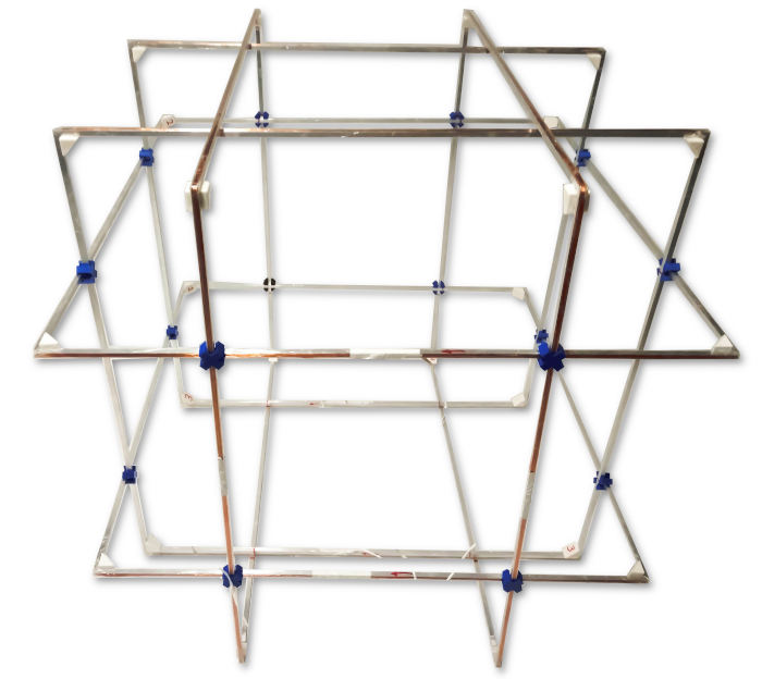 Assembled Helmholtz coils cage
Electronics
We designed custom circuitry to control the current that goes through the 6 coils and therefore the magnitude and direction of the magnetic field.
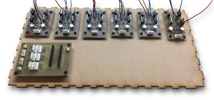 The electronics control circuitry inside the control box (without the wiring)
The subsystems are the following:
- Power H-Bridges (1 per coil): these modules control the amount and the direction of the current that goes through each coil
- Logic computational unit: this board drives the power modules according to the firmware that is loaded on the micro-controller
This circuitry is fitted in a laser-cut control box, with an emergency cutoff switch, 4mm plugs to connect the coils and power supplies, and LEDs for visual indication of the system status.
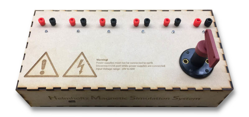 The electronics control box
Power H-bridges
This is the circuit we designed for each these modules:
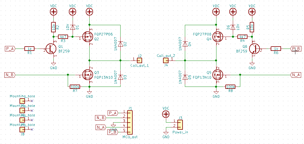 Circuit diagram of the H-bridge module
The interfaces are:
| Signal | Type |
|---|---|
| Coil positive and negative | Power output |
| VDC, GND | Power input |
| P_A, P_B, N_A, N_B | Logic-level input to the transistors |
Using the open-source CAD software KiCad, we designed a single-sided PCB to build 6 identical modules.
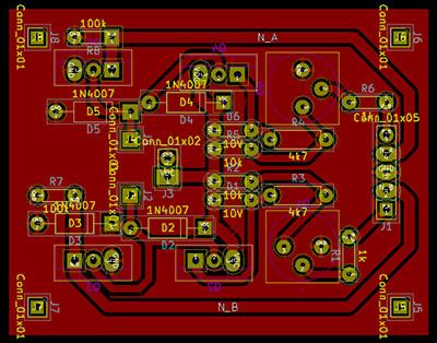 PCB layout of the H-bridge module
This layout is single-sided because it allowed us to do in-house manufacturing of the PCBs, which was a requirement due to time constraints.
Note: to simplify the design, I would recommend using an off-the-shelf integrated circuit such as the DRV8873 instead of this PCB.
Logic unit
The purpose of this board is to run the software and drive the H-bridges. It is based around an Arduino Nano with an Atmel ATMEGA328P mainly because of availability and the simplicity of the programming tool-chain compared to other more powerful micro-controllers.
The interfaces are:
| Connector | Type |
|---|---|
| USB | Communication input |
| H-bridges (×6) | Logic-level output to the transistors |
| LED (×6) | Output to an LED indicator for each coil (PWM) |
We also used KiCad to design a very simple PCB to distribute connectors to the status LEDs and the power modules.
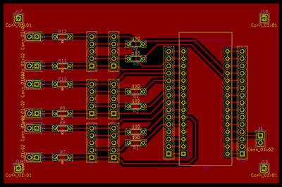 PCB layout of the logic module
We manufactured the modules using both the chemical etching method and a CNC mill.
Software
The Arduino firmware reads the USB serial port, expecting a string with X, Y and Z field values in Gauss. It then handles all of the low level tasks: calculation of the PWM duty cycle, changing the pins’ states, etc. There are also built-in safety procedures to avoid the sudden collapse of the magnetic field, which might be dangerous the electronics.
Example interaction with the device:
> 0 0 0
OK
> 0.2 -0.2 0.5
OK
...
The commands can be manually sent using a serial terminal, but it is intended to be controlled by a higher-level software of the host device (for instance, a Python script that runs the simulation of the fluctuation of the magnetic field over a typical orbit).
Results
To validate our simulator, it is necessary to check two aspects of the magnetic field it generates:
- The constancy of the magnitude with a fixed input current on each of the three axes,
- The control of the field of the field on each of the three axes.
Constancy of the field
To make sure that the field in the working volume is constant, we ran several series of tests. For each of the axes, a constant current is fed into the pair of coils, and a sensor is moved within the cage.
For instance, this capture was taken during a back and forth movement of the sensor along the X axis, while the X axis pair of coils was powered to reach 2.15 Gauss (215 µT).
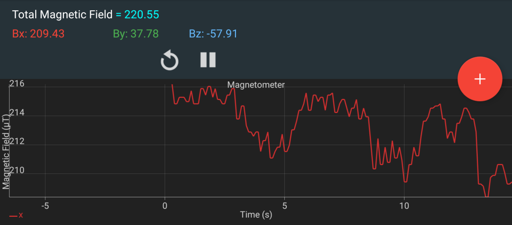 Graph of the variation of the magnetic field in the X axis
The field is very constant: within 0.06 Gauss of variation in the X axis. This matches our specifications.
To give more emphasis on this result, I disconnected the system at t=15s. With the graph re-scaled, this constancy gets more obvious:
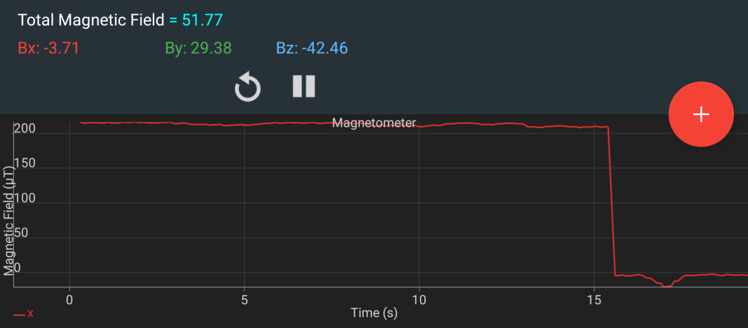 Graph of the variation of the magnetic field in the X axis (longer time)
With the same test performed on the three axes, we validated the constant nature of the magnetic field in our Helmholtz simulation environment. This is a very important result as it proves that the coils are well wound, that the electronics manages to power them with a constant current, and that any testing we will later do in the simulator is meaningful no matter where it is placed in the working volume.
Control of the field
After we is proved that the field is constant within the working zone, we ran another set of test to check that we have full control on the generated field.
The experimental protocol is the following: a description of several magnetic field waveform is done in the software, and a sensor is placed in the Helmholtz coils. If the measured waveform corresponds to the one described in software, it proves that we have control over the magnetic field.
For instance, we asked the software to generate a triangle waveform for the X axis magnetic field. This waveform has an amplitude of 2.15 gauss (215 µT) and a period of 7.5s.
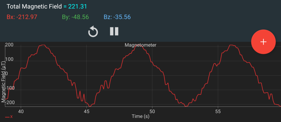 Graph of the variation of the magnetic field in the X axis with a triangular waveform
As shown by this capture, the waveform corresponds to the one we described in software. With the testing of the magnetic field with different waveform in each of the three axes, we validated our control of the Helmholtz simulation environment.
Test with a model CubeSat
We also tested our Helmholtz simulator with a model CubeSat that contains a magnetorquer, a magnetometer, and control board.
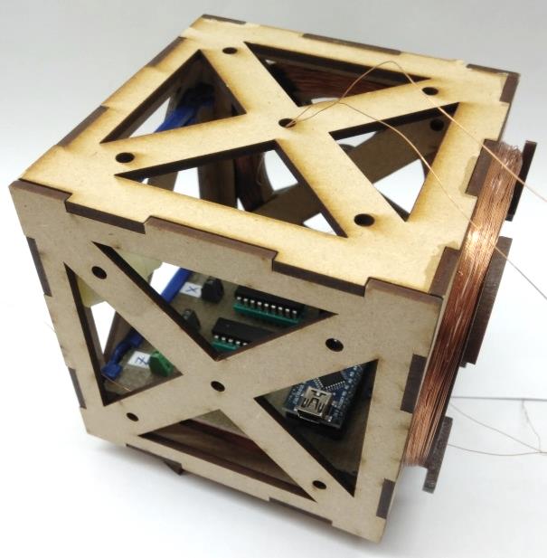 Model of the CubeSat, with 3-axes magnetorquers and logic board.
To achieve this, it is necessary to make a device that allow this model to free spin in every direction. We 3D-printed a large 3 axis gimbal, but is proved very difficult to balance.
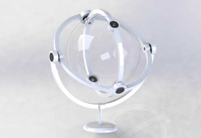 SolidWorks render of the 3 axes CubSat gimbal
We tried to use an air bearing, but it requires a large flow of high pressure air to continuously run. Our compressor could keep up, but it ran its loud motor to do so after a couple minutes of use. Also, the turbulent flow of air that lifts the sphere creates some oscillations, which are a source of error in the simulation.
In the end, we used a simple water bearing. The balanced sphere containing the model floats in a basin:
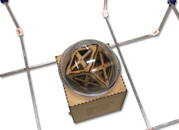 The CubeSat model placed on the water bearing
This solution allowed us to test magnetometers and magnetorquer as long as the model is properly balanced.
Resources
This archive contains Helmholtz coil resources (more design details, code, electronic schematics, etc.). Click on this button to download it:
Notice: the content of this archive is provided "as-is", under the terms of the CC0 1.0 Universal (CC0 1.0) Public Domain Dedication license.
Bibliography/references
- Hurtado, A., García-Farieta, J.E (2019). Simulation of charged particles in Earth's magnetosphere: an approach to the Van Allen belts , Revista Mexicana de Física. https://doi.org/10.31349/RevMexFisE.65.64
Auteur : Charles Grassin
What is on your mind?
#1 ilya
on November 7 2018, 14:15
#2 Alyanna
on November 7 2018, 20:22
#3 Author Charles
on November 7 2018, 21:53
#4 Alyanna
on November 10 2018, 7:08
#5 Author Charles
on November 10 2018, 9:58
#6 Ned
on November 19 2018, 2:51
#7 Author Charles
on November 19 2018, 18:32
#8 Carlos
on March 5 2019, 15:48
#9 Author Charles
on March 5 2019, 19:05
#10 Melvyn
on March 19 2019, 10:06
#11 Author Charles
on March 20 2019, 7:44
#12 Melvyn
on March 20 2019, 9:45
#13 Author Charles
on March 20 2019, 11:19
#14 Melvyn
on March 21 2019, 9:53
#15 Nicolas
on March 26 2019, 15:06
#16 Author Charles
on March 27 2019, 22:35
#17 Melvyn
on March 28 2019, 10:36
#18 RJS
on October 9 2020, 2:20
#19 Author Charles
on October 12 2020, 13:40
#20 RJS
on January 3 2021, 2:45
#21 Jay
on February 8 2021, 10:42
#22 Author Charles
on February 13 2021, 17:08
#23 RJS
on March 17 2021, 15:39
#24 Alex
on March 22 2021, 21:18
#25 Author Charles
on March 24 2021, 9:38
#26 Author Charles
on March 24 2021, 9:43
#27 RJS
on May 30 2021, 3:50
#28 Victoria
on April 25 2023, 13:32
#29 Author Charles
on April 26 2023, 15:39